1. Overview
BrUMaRe reads the outputs of CASTEP [1], VASP and SIESTA and produces, for any material and any atom:
- the band structure, DOS and PDOS, with spin up and down;
- orbital-projected bands;
- the analysis of the local structure of defects (vacancy, substitutional or interstitial) and of the distortion they cause;
- the thermodynamics of formation and of hydrogen desorption;
- the total and spin-polarized charge density, in 3D, 2D and along profiles;
- a side-by-side comparison of several calculations.
There are two ways of using it, which perform the same analysis:
| Website (browser) | Python script (cluster) | |
|---|---|---|
| How to use | drop the files; adjust everything on screen | python3 brumare.py seed |
| Installation | none; the files never leave your computer | Python 3.8+, numpy and matplotlib |
| Outputs | PNG/SVG figures, .dat for Origin, CHGCAR/XSF for VESTA, .zip of calculations, .txt reports | the same, in seed_plots/ |
Core principle: the Fermi energy is never recalculated. The value used is exactly the one the code wrote, for each spin. By default, bands and DOS keep their original energies and a dash-dot line marks EF; E − EF can also be chosen.
Ways to use BrUMaRe
The name BrUMaRe joins Bruno Macedo and Renata Benedet, and it is also the acronym of Brillouin-zone Utilities for Materials Research. Inside it is bruma, Portuguese for mist: the electron cloud the program shows. The same analysis is available in four ways:
| Form | For whom | How to start |
|---|---|---|
| Web page | interactive analysis, nothing to install | open brunohdmacedo.tech/brumare and drop the files |
| Desktop application | the same interface as this page, in a window, offline | pip install "brumare[gui]" and brumare-gui |
| Windows program | the same application, for those who do not use Python | installer BrUMaRe-Setup.exe on the releases page |
| Command line | clusters and scripts | pip install brumare or brumare.py; then brumare mgh2_Fe |
The desktop application and the .exe open this same interface, with the same tabs and exports, using bundled libraries: they work offline. The command line also does the comparison (brumare --comparar A,B,C) and the density-difference report (--field diff). Every form has an About section with name, version, author, links and how to cite; on the command line, use brumare --sobre. The interface is available in Portuguese, English, Spanish, French, Italian and Latin (--idioma on the command line).
Supported codes: CASTEP, VASP and SIESTA
BrUMaRe reads the outputs of the three codes and converts everything to the same internal format. Bands, DOS, PDOS, electronic analysis, defects, thermodynamics, density and comparison work the same way for all three, and calculations from different codes can be compared in the same table. The Fermi energy is always the one the code wrote.
| Code | Files | How to generate |
|---|---|---|
| CASTEP | seed.bands, .pdos_bin, .castep, .cell, .den_fmt | section 2 of this tutorial |
| VASP | the calculation folder: vasprun.xml, KPOINTS, CHGCAR (and POSCAR/CONTCAR) | LORBIT = 11 (projections), ISPIN = 2 (spin), LCHARG = .TRUE. (density); KPOINTS in line mode for bands |
| SIESTA | SystemLabel.bands, .EIG, .KP, .PDOS, .STRUCT_OUT or .XV, .RHO and the .out output | %block BandLines (or BandPoints), %block ProjectedDensityOfStates, SaveRho true, Spin polarized |
How to load:
- In the browser: drop the whole folder or use Open folder. In VASP, the folder name becomes the calculation name, because the files have fixed names. Without a folder, rename the files as
name.vasprun.xml,name.KPOINTSand so on. - In Python:
brumare vasp_folder/,brumare SystemLabel(SIESTA) or simplybrumareinside the folder. In the graphical interface, choose the folder and the calculation from the list.
What changes with each code:
- VASP:
- The projections only cover the PAW spheres around the atoms, so the sum of the PDOS stays below the total DOS. This is normal.
- For a non-self-consistent band calculation, VASP itself recommends using EF from the self-consistent run: load both and choose the self-consistent one in DOS from.
- In non-collinear calculations, only the total part of the projections is used.
- SIESTA:
- The
.PDOScontains the PDOS already computed by SIESTA, with the n, l and m shells and the broadening chosen in the.fdf. It is used directly. - Since there are no band weights, there are no projected bands.
- With
.bandsand.EIGtogether, the bands come from the path and the DOS from the self-consistent mesh, chosen automatically.
- The
- CASTEP only: the Mulliken population and the reference-calculation generator, which writes
.celland.param.
2. Prepare the calculation in CASTEP
.param keywords that produce everything the tool uses:
TASK                    : SPECTRAL           ! or GeometryOptimization, SinglePoint
SPECTRAL_TASK           : BANDSTRUCTURE      ! DOS for a dense mesh
SPIN_POLARIZED          : TRUE
PDOS_CALCULATE_WEIGHTS  : TRUE               ! writes the .pdos_bin (PDOS and projected bands)
POPN_CALCULATE          : TRUE               ! Mulliken and bonds in the .castep
WRITE_FORMATTED_DENSITY : TRUE               ! writes the .den_fmt (charge and spin density)
The band path goes in the .cell, in %BLOCK SPECTRAL_KPOINT_PATH [5]. For a quantitative DOS, run a second calculation with SPECTRAL_TASK : DOS and a dense Monkhorst–Pack mesh [3]; then select that calculation in DOS from.
| File | Used for |
|---|---|
seed.bands | eigenvalues, EF of each spin, k-point weights and cell: bands, DOS and gap |
seed.pdos_bin | weight of each orbital in each band and k-point: PDOS and projected bands |
seed.castep | shells (2p, 3d…), m orbitals, Mulliken [6][7], bonds, energies, forces, valence Z |
seed.cell | species order, defect structure, basis to generate the references |
seed.den_fmt, .cube, CHGCAR | charge and spin density |
3. Open the files
- Open the tool and drop the files on the dashed area, or click Open files.
- Each seedname is a calculation. You can load several at once: the defect, the pure structure, the elemental references and other dopants.
- Use × next to a calculation to remove it, or Clear data to start over.
- The ☀/☾ button switches the theme; the choice also applies to the portfolio. The language selector is next to it.
4. Bands
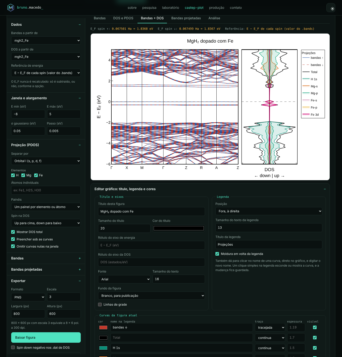
The Bands tab shows spin up and down overlaid, side by side or only one of them. The labels of the high-symmetry points are detected for cubic, tetragonal, orthorhombic and hexagonal lattices, or typed in k-point labels (for example G,X,M,G,Z,R,A,Z).
By default the energy axis keeps the original energies, with a dash-dot line and the value of EF; the reference can also be the EF of each spin or a common EF (E − EF).
5. DOS and PDOS
The DOS is the sum of Gaussians over bands and k-points, with the chosen broadening σ. The PDOS can be split into five levels:
| Level | Example |
|---|---|
| Element | Mg, H, Fe |
| Orbital l | Fe-s, Fe-p, Fe-d |
| Pseudopotential shell (n, l) | Mg 2p and Mg 3p |
| m component | px, py, pz, dz², dyz, dxz, dx²−y², dxy |
| t2g/eg and individual atoms | Fe 3d t2g; Fe1, H25 |
The Bands + DOS tab places both plots side by side, on the same energy axis.
6. Projected bands
In projected bands, the size of each point is proportional to the orbital weight in that band and k-point. They use the projections chosen in the Projection section, in separate or overlaid panels.
7. Electronic analysis
The Analysis tab gathers, for each spin:
- EF in Ha and in eV;
- VBM and CBM, defined by electron counting (bands N and N+1), and the direct or indirect gap with its k-points;
- whether EF falls inside a band;
- N(EF) and the spin polarization;
- the integrated spin;
- the integrated PDOS occupations and the d-band center;
- Mulliken per species and per atom;
- the dopant bonds.
8. Plot editor
Right below each figure is the Edit plot: title, legend and colors panel:
- Title and axes: title, size, color, axis labels, font and background (white for publication or site colors).
- Legend: position, size, title and frame.
- Curves: for each curve, color, legend name, dash, width and visibility.
- Directly on the plot: click a legend name to edit it. Edits apply to all tabs.
9. Defect and distortion
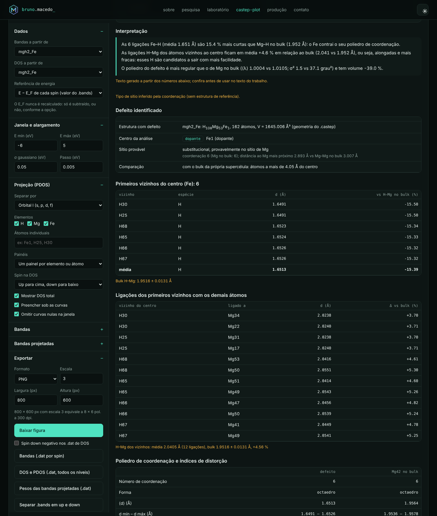
The Defect and thermodynamics tab identifies the defect in two ways:
- With the pure reference structure: each atom is matched to its site, with periodic boundary conditions, and the type (vacancy, substitutional or interstitial) is found automatically.
- Without a reference: the defect is compared with the "bulk" of the supercell itself, that is, with the atoms far from it.
It computes:
- first neighbors: each X–H bond, for example, against the reference and against Mg–H in the bulk;
- neighbor bonds (for example H–Mg);
- polyhedron distortion indices: Baur [9], ECoN [10], quadratic elongation ⟨λ⟩ and angle variance σ² [8], volume and angles;
- second shell;
- with the reference: the displacement field and the perturbation radius.
10. Thermodynamics
The chemical potentials μi are the energies per atom of the elemental references, computed with the same parameters: hcp Mg, bcc Fe and \(\mu_\mathrm{H}=\tfrac12E(\mathrm{H_2})\). When the .castep of these references is loaded, they are filled in automatically.
It computes:
- the defect formation energy [16][17];
- the hydride formation enthalpy per mole of H₂, and the defect effect ΔΔH;
- the desorption temperature from van ’t Hoff, with ΔS ≈ standard entropy of gaseous H₂ [19];
- the H removal energy;
- the gravimetric capacity.
The formulas are in section 18.
11. Generate the reference calculations
With Generate the reference calculations from this .cell, the tool writes .cell and .param files with the same functional, cutoff, spin, tolerances and pseudopotentials as your calculation:
| Calculation | Use |
|---|---|
seed_puro | pure structure (relax) |
seed_dif_puro_fixo | pure host in the defect geometry (single point): Δρ without relaxation dipoles |
seed_dif_sem_X, seed_dif_so_X | without the dopant and only the dopant, in the same cell (single point): bonding density |
seed_semH_perto, seed_semH_longe | H removal energy near and far from the defect |
Mg_hcp, Fe_bcc, H_H2… | chemical potentials μ |
The supercells use exactly the same k mesh as the defect. The elemental references use the same k-point density.
12b. Brillouin zone and k-path
The Brillouin zone tab computes the first zone (the Wigner–Seitz cell of the reciprocal lattice) of any crystal, finds the high-symmetry points, builds the band path and writes ready-to-use inputs for the calculation.
- Choose the structure: a loaded calculation, one of the examples (Si, Cu, Fe, Mg, rutile, MgH₂…) or a lattice typed by hand (a, b, c, α, β, γ or the three vectors).
- Symmetry tolerance: with “Symmetrize the lattice”, nearly equal angles and lengths are adjusted (default 0.5° and 0.5%), as SeeK-path does. A relaxed cell with γ = 89.75° is then treated as tetragonal; the adjustments are shown on screen.
- Path density and Δk: set the number of points per segment and the suggested Monkhorst–Pack meshes (nᵢ = ⌈|bᵢ|/Δk⌉).
- Result: 3D zone (volume, edges, points, path and b₁, b₂, b₃), lattice type, volumes, vectors, table of points (fractional and Cartesian), segment lengths and meshes.
- Ready inputs: CASTEP (
SPECTRAL_KPOINT_PATHandKPOINTS_MP_GRID), VASP (line-modeKPOINTS), Quantum ESPRESSO (K_POINTS crystal_b), SIESTA (BandLines) and JSON, with Copy and Download buttons. - Command line:
brumare --zona-brillouin "fcc 5.431"orbrumare seed --zona-brillouinwrite the report, the input files, the JSON and the figure.
Symmetry and structures. With atoms (a loaded calculation, a CIF/POSCAR/.cell/XSF/QE/XYZ file, a COD number or the library of 51 literature materials), the tab identifies the space group with moyo, the successor of spglib (used by SeeK-path): number, Hermann–Mauguin and Hall symbols, Pearson symbol, crystal system, Bravais lattice, point group, operations, inversion and the Wyckoff positions of every atom. The zone and points then use the standardized primitive cell, which can be exported (as can the conventional cell) as POSCAR, .cell, QE and CIF. With a structure, all 14 Bravais lattices (the 25 Setyawan–Curtarolo cases, from CUB to TRI) get their standard points and paths, checked against pymatgen; without atoms, low-symmetry lattices get an automatic path. Command line: brumare --estrutura file.cif.
Fractional coordinates refer to the reciprocal basis of the chosen cell: use the same cell in the calculation. For supercells the zone is smaller and the bands are folded; for the standard path of the material, use the primitive cell. Cubic, FCC, BCC, hexagonal, tetragonal and orthorhombic lattices get the labels and paths of Setyawan and Curtarolo (2010); for low-symmetry lattices the path is automatic (Γ to each face centre) and SeeK-path (Hinuma et al., 2017) is recommended.
12. Charge density
In the 3D structure and density tab, the available quantities are total ρ, ρ↑, ρ↓, ρ↑ − ρ↓, |ρ↑ − ρ↓|, ζ = (ρ↑ − ρ↓)/ρ and Δρ.
- 3D: adjustable isosurface, with atoms, bonds and cell.
- 2D: slices through a plane.
- Profile: density along a bond, with the minimum that approximates the bond critical point.
- Charges and moments per atom: Voronoi partition [12], standard or radical [13], and a sphere around the defect.
- For VESTA [15]: export CHGCAR (VASP 5 format with the elements, ρ·V) or XSF. The CHGCAR also works with the
baderprogram [14].
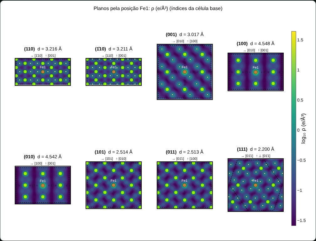
13. (h k l) planes, gallery and cell
- Base-cell indices: the tool detects the supercell multiplicity (for example 3×3×3 of rutile MgH₂), and the indices are those of the material.
- Natural axes: the slice axes follow lattice directions; for (110), horizontal [1̄10] and vertical [001].
- Whole section: the slice covers the whole supercell section, with the cell outline.
- Sweep: a control shifts the plane along its normal.
- Gallery: shows (110), (1̄10), (001), (100), (010), (101), (011) and (111) side by side.
- Cell panel: density, H capacity, coordination, distances per pair and dhkl spacings.
14. Defect contribution: Δρ
To see only the effect of the defect, choose Quantity → defect contribution and, in Subtract ρ(B), the density of the pure material (it is chosen automatically when its name contains "puro"). There are three ways, from the simplest to the cleanest:
- ρ(defect) − ρ(relaxed pure): includes the electronic effect and the relaxation. Dipoles appear around the atoms that moved.
- ρ(defect) − ρ(pure in the defect geometry), with
seed_dif_puro_fixo: same grid and same positions. It shows only the replacement of the host by the dopant. - ρ(defect) − ρ(without the dopant) − ρ(only the dopant), with B and C: the dopant bonding density, that is, the charge redistribution upon forming the bonds.
If the grids differ, the subtracted density is resampled on the defect grid. The tool shows:
- the electrons gained and lost and the balance;
- ∫Δρ in spheres around the dopant;
- the charge transfer per atom (∫Δρ in the Voronoi cell of each atom).
Components and sign. The difference can be taken for the total (Δρ), for each spin (Δρ↑, Δρ↓) and for the magnetization, Δ(ρ↑ − ρ↓). In Sign of the difference, choose ρ(defect) − ρ(pure) or ρ(pure) − ρ(defect). Positive values are red and negative values blue. Use Color scale limit ± to highlight the weak redistribution on the neighbors.
3D around the defect. In 3D region, a box of ±3 to ±6 Å centered on the dopant shows the Δρ lobes with the bonds.
Comparison and VESTA. In the Comparison tab, the difference of each defect against the reference appears in 3D, side by side, and in 2D on the same plane. The Export to VESTA: all calculations button creates a .zip with one folder per structure. Each folder has the CHGCARs of ρ, ρ↑, ρ↓, ρ↑ − ρ↓ and of the four differences, with the correct elements and positions, plus a guide with the value range and a step-by-step for VESTA.
Density difference tab
A report dedicated to the charge redistribution caused by the defect, with:
- indicators: ΔN, accumulation, depletion and redistributed charge ½∫|Δ|; 50% and 90% radii; points of maximum accumulation and depletion; redistribution dipole (\(\mathbf p=\int(\mathbf r-\mathbf r_c)\,\Delta\rho\,dV\), in e·Å and Debye); change of the moment;
- bonds: minimum ρ of each dopant–neighbor bond against the same host bond in the pure structure;
- charge per atom in both structures, with matched atoms;
- triptychs ρ(pure) | ρ(defect) | Δρ, in 2D and 3D;
- radial profile ⟨Δ⟩(r) with the accumulated charge \(\Delta Q(r)=\int_0^r\Delta\rho\,4\pi r'^2dr'\);
- planar averages along a, b and c;
- profile along the bond.
Everything can be exported to Origin and VESTA.
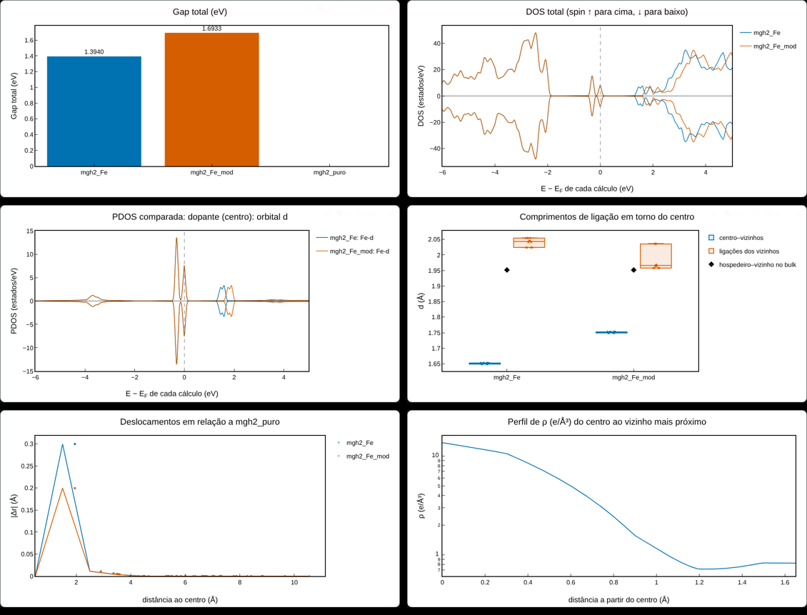
15. Comparison between calculations
In the Comparison tab, tick the calculations and, if available, the pure reference structure. You get:
- a table with one column per calculation: energies, Ef, ΔH, ΔΔH, Td, EF, gaps, N(EF), polarization, d occupation and moment, Mulliken, Voronoi, ρ at the critical point, coordination, bonds, ⟨λ⟩, σ², displacements, ΔV/V, cell and residual force;
- plots: bars, overlaid DOS and PDOS, bands side by side, bonds, displacements, density (including Δρ against the reference) on the same plane and profiles.
16. Exports
| Output | Format | Use |
|---|---|---|
| Figures | PNG, JPG, JXL (JPEG XL), WEBP, SVG (scale 3 = 300 dpi at 8×6 in) | papers, theses, dissertations |
| Bands, DOS/PDOS, weights, slices, profiles, comparison | .dat with TAB and a header line | Origin, Excel, gnuplot |
| Density | CHGCAR (VASP 5), XSF | VESTA, Bader, XCrySDen |
| Reference calculations | .zip with .cell, .param, README, script | cluster |
.bands per spin | seed_up.bands, seed_down.bands | sumo [18] and others |
| Reports | .txt | analysis, defect, comparison |
| Citation | brumare_citacao.bib | BrUMaRe, the codes and the methods you used |
In Origin: drag the .dat; the header line becomes the Long Name of each column. For bands, column 1 is X; plot the others as lines.
17. Python script
# everything: bands, DOS/PDOS, analysis, defect, density, structure
python3 brumare.py mgh2_Fe -e Mg,H,Fe
# defect with reference and thermodynamics
python3 brumare.py mgh2_Fe --ref mgh2_puro --mu "Mg=@Mg_hcp,Fe=@Fe_bcc,H=@H_H2" --h-less mgh2_Fe_semH_perto
# generate the reference calculations
python3 brumare.py mgh2_Fe --gerar-referencias
# density: plane gallery, spin, CHGCAR for VESTA
python3 brumare.py mgh2_Fe --planes todos --field spin --chgcar
# defect contribution and charge transfer per atom
python3 brumare.py mgh2_Fe --field diff --subtract mgh2_Fe_dif_puro_fixo.den_fmt
# VESTA package: ρ, ρ↑, ρ↓, spin and the differences (pure − defect)
python3 brumare.py mgh2_Fe --vesta --subtract mgh2_puro.den_fmt --diff-sign puro-defeito
# texts (--sobre, citation) in English
python3 brumare.py mgh2_Fe --idioma en
Use python3 brumare.py -h for all options.
18. Formulas
DOS, with weights \(w_k\) and Gaussian broadening \(\sigma\):
\[ g_s(E)=\sum_{k}w_k\sum_n \frac{1}{\sigma\sqrt{2\pi}}\exp\!\left[-\frac{(E-\varepsilon_{nks})^2}{2\sigma^2}\right],\qquad g^{\mathrm{PDOS}}_{s,\alpha}(E)=\sum_k w_k\sum_n p^{\alpha}_{nks}\,\delta_\sigma(E-\varepsilon_{nks}) \]
Gap, with \(N\) the number of electrons per spin: \(E_g=\min_k\varepsilon_{N+1,k}-\max_k\varepsilon_{N,k}\). Polarization: \(P=\dfrac{N_\uparrow(E_F)-N_\downarrow(E_F)}{N_\uparrow(E_F)+N_\downarrow(E_F)}\).
Polyhedron distortion [9][10][8]:
\[ D=\frac1n\sum_i\frac{|d_i-\bar d|}{\bar d},\qquad \langle\lambda\rangle=\frac1n\sum_i\left(\frac{d_i}{l_0}\right)^2,\qquad \sigma^2=\frac{1}{m-1}\sum_j(\theta_j-\theta_0)^2,\qquad \mathrm{ECoN}=\sum_i e^{\,1-(d_i/d_\mathrm{av})^6} \]
Here \(l_0\) is the center–vertex distance of the regular polyhedron of the same volume and \(\theta_0\) is 90° (octahedron) or 109.47° (tetrahedron).
Thermodynamics [16]:
\[ E_f=E_\mathrm{def}-E_\mathrm{pure}-\sum_i n_i\mu_i,\qquad \Delta H_f=\frac{E-\sum_i N_i\mu_i}{N_\mathrm{H}/2},\qquad T_d=\frac{\Delta H}{\Delta S},\qquad \mu_\mathrm{H}=\tfrac12E(\mathrm{H}_2) \]
In Ef, \(n_i>0\) indicates added atoms. ΔH is per mole of H₂ and the standard ΔS is 130.7 J/(mol·K).
Density: CASTEP and VASP write \(\rho V\). BrUMaRe uses \(\rho\) in e/ų, with \(\int\rho\,dV=N_e\), \(\zeta=(\rho_\uparrow-\rho_\downarrow)/\rho\) and \(\Delta\rho=\rho_A-\rho_B-\rho_C\). In the radical Voronoi partition, each point goes to the atom that minimizes \(|\mathbf r-\mathbf R_a|^2-r_a^2\), with Cordero’s covalent radii [11].
18b. Complete theory and examples
Every quantity BrUMaRe computes, with the equation used, and a real example for each code, so you can check that your result makes sense.
Units and reading of each code
| Code | What is read | Conversion |
|---|---|---|
| CASTEP | .bands (Ha), .pdos_bin, .castep, .den_fmt (ρV) | \(1\,\mathrm{Ha}=27.211386\,\mathrm{eV}\); \(1\,\mathrm{Bohr}=0.529177\,\text{Å}\) |
| VASP | vasprun.xml (eV), PAW projections, CHGCAR (ρV) | energies already in eV; \(\rho=\mathrm{CHGCAR}/V\) |
| SIESTA | .bands, .EIG (eV), .PDOS ready-made, .RHO (e/Bohr³) | \(\rho\,[\mathrm{e/\text{Å}^3}]=\rho\,[\mathrm{e/Bohr^3}]/0.529177^3\) |
| Quantum ESPRESSO | data-file-schema.xml (Ha; k em \(2\pi/a\)) | \(\mathbf k_\mathrm{frac}=\mathbf k_\mathrm{cart}\cdot\mathbf A^{T}/(2\pi)\) |
| ORCA | .out output: orbitals, energy, geometry, charges | molecule: a single "k-point"; DOS from Gaussians on the levels |
Bands, gap and effective mass
With \(N_s\) electrons in spin \(s\), the last occupied band is \(N_s\) and the first empty one is \(N_s+1\): \(E_\mathrm{VBM}=\max_k\varepsilon_{N_s,k}\), \(E_\mathrm{CBM}=\min_k\varepsilon_{N_s+1,k}\) e \(E_g=E_\mathrm{CBM}-E_\mathrm{VBM}\). For molecules (ORCA), the same criterion gives the HOMO–LUMO gap.
The effective mass comes from a parabolic fit around the extremum, along the path:
\[ E(k)\approx E_0+\frac{\hbar^2 (k-k_0)^2}{2m^*}\quad\Rightarrow\quad \frac{m^*}{m_e}=\frac{\hbar^2}{2m_e\,c_2},\qquad \frac{\hbar^2}{2m_e}=3.80998\ \mathrm{eV\,\text{Å}^2} \]
At a vertex (such as Γ), one mass is given for each path direction. It is only computed when EF lies in the gap and the path is continuous.
DOS, PDOS and Fermi level
\[ g_s(E)=\sum_k w_k\sum_n \frac{e^{-(E-\varepsilon_{nks})^2/2\sigma^2}}{\sigma\sqrt{2\pi}},\qquad N_s(E_F)=g_s(E_F),\qquad P=\frac{N_\uparrow-N_\downarrow}{N_\uparrow+N_\downarrow} \]
EF is always the value written by the code. By default, the axis shows the original energies and a dash-dot line marks EF; the E min/E max window is counted from EF. The polarization is only defined when \(N_\uparrow+N_\downarrow>0.05\) states/eV.
d-band center: \(\varepsilon_d=\int E\,g_d(E)\,dE\big/\int g_d(E)\,dE\), up to EF (occupied) or over the whole window.
Brillouin zone
The zone is built from the Bragg planes k·G = |G|²/2 on a reduced (LLL) reciprocal basis; its geometric volume is checked against (2π)³/V, and the lattice type is recognised from the shape of the zone (number and shape of the faces).
\[ \mathbf b_1=2\pi\frac{\mathbf a_2\times\mathbf a_3}{V},\quad \mathbf a_i\cdot\mathbf b_j=2\pi\delta_{ij},\quad V_\mathrm{ZB}=\frac{(2\pi)^3}{V},\quad \mathbf k\cdot\mathbf G\le\tfrac12|\mathbf G|^2\ \ \forall\,\mathbf G,\quad k_i^\mathrm{frac}=\frac{\mathbf a_i\cdot\mathbf k}{2\pi},\quad n_i=\left\lceil\frac{|\mathbf b_i|}{\Delta k}\right\rceil \]
Band-gap correction (scissor)
LDA and GGA functionals (such as PBE) underestimate the gap because the Kohn–Sham gap is not the fundamental gap: the derivative discontinuity of the exchange-correlation functional is missing and there is delocalisation error. BrUMaRe offers a post-processing correction: the scissor rigidly shifts the unoccupied bands (\(n>N_s\)) by \(\Delta\), leaving the occupied bands and EF unchanged. \(\Delta\) can be given, computed from a reference gap (experimental, HSE06 or GW) or estimated with the empirical PBE → G0W0 model of Morales-García, Valero and Illas (2017), fitted on 66 solids.
\[ E_g^\mathrm{DFT}=E_\mathrm{CBM}-E_\mathrm{VBM},\qquad \varepsilon^\mathrm{corr}_{n\mathbf k s}=\varepsilon_{n\mathbf k s}+\Delta\,\Theta(n-N_s),\qquad \Delta_\mathrm{ref}=E_g^\mathrm{ref}-E_g^\mathrm{DFT},\qquad E_g^{G_0W_0}\approx 1.358\,E_g^\mathrm{PBE}+0.904\ \mathrm{eV} \]
Limits: the scissor does not correct band dispersion, effective masses or the position of empty defect levels in the gap; the empirical model applies to PBE (not LDA), requires a non-zero gap and errs by a few tenths of an eV (Si: 1.74 eV estimated versus 1.17 eV experimental). In defective supercells, prefer the Δ of the pure material. For a real correction, recompute with HSE06, rSCAN or DFT+U. Command line: --gap-corr mvi, --gap-corr ref --gap-ref 1.17 or --gap-corr tesoura --tesoura 0.5.
Charges: Mulliken, Voronoi and Bader
- Mulliken (CASTEP and ORCA): read from the code output; charge \(q_a=Z_a-N_a\).
- Voronoi: \(N_a=\int_{V_a}\rho\,dV\), with \(V_a\) the points closest to atom \(a\) (or, in the radical version, those minimizing \(|\mathbf r-\mathbf R_a|^2-r_a^2\)).
- Bader [14]: each grid point follows the gradient of ρ up to a maximum (Henkelman’s on-grid algorithm); the basins ending at the same atom add up to \(N_a\). Magnetic moment: \(m_a=\int_{V_a}(\rho_\uparrow-\rho_\downarrow)\,dV\) in μB. On the command line, basin boundaries are refined with the near-grid method (Tang, Sanville and Henkelman, 2009), which follows the true gradient of ρ and removes the lattice bias; the result differs from the reference implementation (pybader) by less than 0.001 e per atom on average.
Defect, distortion and thermodynamics
\[ E_f=E_\mathrm{def}-E_\mathrm{puro}-\sum_i n_i\mu_i,\qquad \Delta H=\frac{E-\sum_iN_i\mu_i}{N_\mathrm H/2},\qquad T_d=\frac{\Delta H}{\Delta S},\qquad \langle\lambda\rangle=\frac1n\sum_i\Big(\frac{d_i}{l_0}\Big)^2 \]
Density and density difference
\[ \Delta\rho=\rho_\mathrm{def}-\rho_\mathrm{ref}\ [-\rho_C],\qquad Q_\mathrm{red}=\tfrac12\!\int|\Delta\rho|\,dV,\qquad \mathbf p=\int(\mathbf r-\mathbf r_c)\Delta\rho\,dV,\qquad \Delta Q(r)=\int_0^r\overline{\Delta\rho}\,4\pi r'^2dr' \]
Real examples (one per code)
Results obtained with real output files; use them to check your installation.
| Code and system | Command | Result |
|---|---|---|
| CASTEP · MgH₂:Fe (162-atom supercell, spin) | brumare mgh2_Fe -e Mg,H,Fe | EF = 1.837 eV; total gap 1.394 eV, indirect M→R; Fe–H 1.649–1.653 Å |
| VASP · Si (line-mode bands) | brumare Si_bands/ | gap 0.614 eV indirect (Γ→near X); m*e = 0.94 me; m*h(Γ) = 0.32 me |
| VASP · Fe₂O₃ ferromagnetic (LDA+U) | brumare FeO_ldau/ | 56 electrons ↑ and 36 ↓: moment 20 μB (4 high-spin Fe³⁺) |
| SIESTA · SrTiO₃ | brumare SrTiO3 | gap 2.25 eV indirect R→Γ; O 2p in the valence band; Ti 3d t2g/eg in the conduction band; ∫ρ = 40.000 e |
| Quantum ESPRESSO · Si | brumare folder_with_xml/ | gap 1.32 eV between the 2 test k-points (coarse mesh) |
| ORCA · divinylbenzene (molecule) | brumare dvb_sp.out | HOMO–LUMO gap 5.18 eV; Mulliken and Löwdin charges |
| Comparison between codes | brumare --comparar mgh2_Fe,Si_bands/,SrTiO3 | comparacao.dat table, overlaid DOS, bands side by side and comparacao_citacao.bib |
19. Caveats and limitations
- DOS from the band path is only illustrative; for numbers, use a dense mesh.
- Gap and edges come only from the k-points of the path.
- m components and t2g/eg are in the Cartesian axes of the cell.
- 0 K energies have no zero-point energy; Td is an estimate for comparing trends.
- Same parameters: compare only calculations with the same functional, cutoff, pseudopotentials and U.
- Voronoi charges are estimates; for quantitative numbers, use Bader.
- Δρ with different grids or volumes is resampled. Identical grids, with
dif_puro_fixo, are ideal.
20. How to cite
If BrUMaRe helped your work, cite the software and, when relevant, the author’s bachelor thesis and dissertation. Also cite CASTEP [1] (or VASP or SIESTA) and VESTA [15], if you used it. The Cite (.bib) button in the tool downloads a .bib with exactly what you used. Downloads: brumare.bib · CITATION.cff · tutorial in PDF · LaTeX source.
ABNT (NBR 6023)
Citations are kept in their original language, as published.
BibTeX
@misc{macedo2026brumare,
  author       = {Macedo, Bruno Henrique Dourado},
  title        = {{BrUMaRe}: {Brillouin-zone Utilities for Materials Research} --- análise de estrutura de bandas, {DOS}, {PDOS}, densidade de carga, defeitos e termodinâmica a partir de cálculos {CASTEP}, {VASP} e {SIESTA}},
  year         = {2026},
  version      = {1.3.0},
  howpublished = {\url{https://brunohdmacedo.tech/brumare/}},
  note         = {Código-fonte: \url{https://github.com/brunohdmacedo/brumare}}
}@misc{macedo2025tcc,
author = {Macedo, Bruno Henrique Dourado},
title = {Influência de defeitos substitucionais nas propriedades estruturais, eletrônicas, termodinâmicas e de armazenamento do hidreto {MgH$_2$}: uma abordagem \textit{ab initio}},
year = {2025},
howpublished = {Trabalho de Conclusão de Curso (Bacharelado em Engenharia Física), UNILA},
url = {https://dspace.unila.edu.br/items/8db3836e-925d-422f-9cd2-6ff3f9f02080},
note = {Orientador: Rodrigo Santos da Lapa}
}
@misc{macedo2024dataset,
author = {Macedo, Bruno Henrique Dourado and Zalewski, Willian},
title = {Dataset\_Machine\_Learning\_Exoplanets\_2024},
year = {2024},
howpublished = {Mendeley Data, v3},
doi = {10.17632/wctcv34962.3}
}@mastersthesis{macedo2027dissertacao,
author = {Macedo, Bruno Henrique Dourado},
title = {Influência de defeitos substitucionais no {MgH$_2$}: uma abordagem \textit{ab initio}},
school = {PPGFISA, Universidade Federal da Integração Latino-Americana (UNILA)},
address = {Foz do Iguaçu, PR},
year = {2027},
type = {Dissertação (Mestrado em Física Aplicada)},
note = {Orientador: J. R. C. Salgado; coorientador: R. S. da Lapa. Bolsa CNPq}
}O TCC, o artigo e a base de dados foram conferidos no DSpace UNILA, na RBIC e no Mendeley Data; o título da dissertação (em andamento) ainda deve ser conferido. No GitHub, o arquivo CITATION.cff faz aparecer o botão “Cite this repository”.
21. References
- CLARK, S. J. et al. First principles methods using CASTEP. Z. Kristallogr., v. 220, p. 567–570, 2005. doi:10.1524/zkri.220.5.567.65075
- PERDEW, J. P.; BURKE, K.; ERNZERHOF, M. Generalized gradient approximation made simple. Phys. Rev. Lett., v. 77, p. 3865, 1996. doi:10.1103/PhysRevLett.77.3865
- MONKHORST, H. J.; PACK, J. D. Special points for Brillouin-zone integrations. Phys. Rev. B, v. 13, p. 5188, 1976. doi:10.1103/PhysRevB.13.5188
- SAKINTUNA, B.; LAMARI-DARKRIM, F.; HIRSCHER, M. Metal hydride materials for solid hydrogen storage: a review. Int. J. Hydrogen Energy, v. 32, p. 1121–1140, 2007. doi:10.1016/j.ijhydene.2006.11.022
- SETYAWAN, W.; CURTAROLO, S. High-throughput electronic band structure calculations. Comput. Mater. Sci., v. 49, p. 299–312, 2010. doi:10.1016/j.commatsci.2010.05.010
- MULLIKEN, R. S. Electronic population analysis on LCAO–MO molecular wave functions. I. J. Chem. Phys., v. 23, p. 1833, 1955. doi:10.1063/1.1740588
- SEGALL, M. D. et al. Population analysis of plane-wave electronic structure calculations of bulk materials. Phys. Rev. B, v. 54, p. 16317, 1996. doi:10.1103/PhysRevB.54.16317
- ROBINSON, K.; GIBBS, G. V.; RIBBE, P. H. Quadratic elongation. Science, v. 172, p. 567–570, 1971. doi:10.1126/science.172.3983.567
- BAUR, W. H. The geometry of polyhedral distortions. Acta Cryst. B, v. 30, p. 1195–1215, 1974. doi:10.1107/S0567740874004560
- HOPPE, R. Effective coordination numbers (ECoN) and mean fictive ionic radii (MEFIR). Z. Kristallogr., v. 150, p. 23–52, 1979. doi:10.1524/zkri.1979.150.1-4.23
- CORDERO, B. et al. Covalent radii revisited. Dalton Trans., p. 2832–2838, 2008. doi:10.1039/B801115J
- VORONOI, G. Nouvelles applications des paramètres continus à la théorie des formes quadratiques. J. Reine Angew. Math., v. 134, p. 198–287, 1908. doi:10.1515/crll.1908.134.198
- GELLATLY, B. J.; FINNEY, J. L. The radical alternative to the Voronoi polyhedron. J. Non-Cryst. Solids, v. 50, p. 313–329, 1982. doi:10.1016/0022-3093(82)90093-X
- HENKELMAN, G.; ARNALDSSON, A.; JÓNSSON, H. A fast and robust algorithm for Bader decomposition of charge density. Comput. Mater. Sci., v. 36, p. 354–360, 2006. doi:10.1016/j.commatsci.2005.04.010
- MOMMA, K.; IZUMI, F. VESTA 3 for three-dimensional visualization of crystal, volumetric and morphology data. J. Appl. Cryst., v. 44, p. 1272–1276, 2011. doi:10.1107/S0021889811038970
- FREYSOLDT, C. et al. First-principles calculations for point defects in solids. Rev. Mod. Phys., v. 86, p. 253–305, 2014. doi:10.1103/RevModPhys.86.253
- VAN DE WALLE, C. G.; NEUGEBAUER, J. First-principles calculations for defects and impurities. J. Appl. Phys., v. 95, p. 3851, 2004. doi:10.1063/1.1682673
- GANOSE, A. M.; JACKSON, A. J.; SCANLON, D. O. sumo. J. Open Source Softw., v. 3, p. 717, 2018. doi:10.21105/joss.00717
- CHASE, M. W. NIST-JANAF Thermochemical Tables. 4. ed. J. Phys. Chem. Ref. Data, Monograph 9, 1998.